AI Series: Understanding Noise Reduction and Contrast Adjustment
A guide to understanding noise reduction and contrast adjustment in image processing.

What you will learn
- How to introduce salt-and-pepper noise into images.
- How to apply the median filter to eliminate noise + our own method.
- How to adjust the contrast of an image using the histogram equalization technique + our own method.
- How to measure the performance of our methods.
Exploring Salt-and-Pepper Noise
What is Salt-and-Pepper Noise?
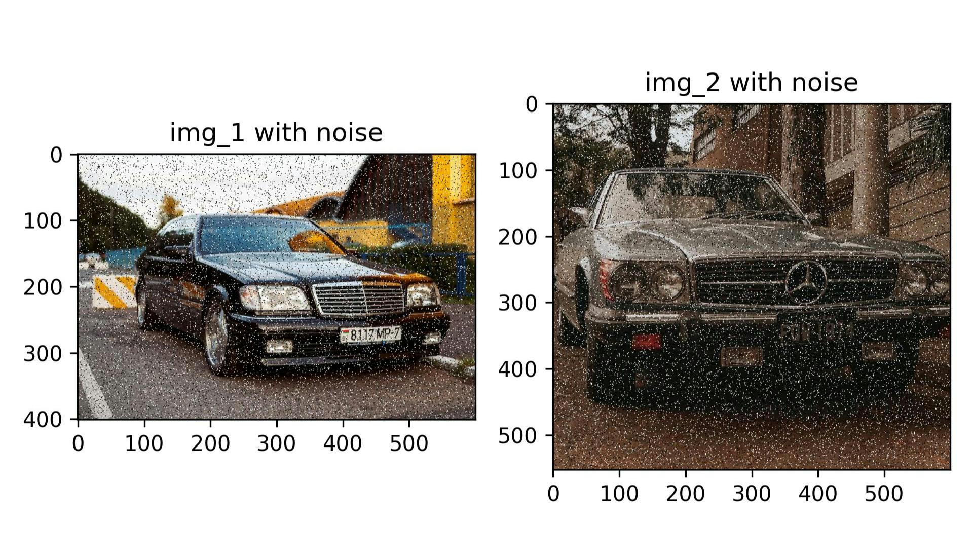
Salt-and-pepper noise is a specific type of noise commonly encountered in digital images. It's characterized by sudden disturbances in the image's brightness, resulting in random black and white pixels. This type of noise can significantly degrade the quality of an image, making it a primary target for noise reduction techniques in image processing.
Generating Salt-and-Pepper Noise
This technique involves randomly altering certain pixels in an image to become either completely white (salt) or completely black (pepper). The process is based on probability, represented in the following scheme:
0                     prob / 2                     1 - prob / 2                 1
|-----------------------|-------------------------------|-----------------------|
      Pepper (Black)                  Neutral                    Salt (White)
Given a random value:
- If it falls between
0andprob / 2, the pixel turns into pepper (black). - Pixels that fall into the intermediate (neutral) range remain unchanged.
- If it falls between
1 - prob / 2and1, the pixel turns into salt (white).
This method allows us to simulate the effect of noise on images in a controlled manner, which is essential for the subsequent phases of our experiment.
Noise Reduction Techniques
The Median Filter Method
The median filter is a well-established technique in image processing, renowned for its effectiveness in reducing salt-and-pepper noise. Unlike mean filters, which often blur an image, median filters preserve edges while removing noise, making them particularly useful in maintaining the structural integrity of an image.
How Median Filters Work
- Kernel Size Selection: First, choose a kernel size (typically an odd number like 3x3, 5x5, etc.). The kernel size determines the area around each pixel to consider for filtering.
- Pixel-by-Pixel Analysis: The filter moves across the image, analyzing each pixel.
- Neighborhood Examination: For each pixel, it examines the intensity values of neighboring pixels within the kernel.
- Median Calculation: The median of these values is computed and replaces the original pixel value.
OpenCV Implementation
import cv2 as cv

def median_filter_cv(img, kernel_size):
    return cv.medianBlur(img, kernel_size)
This function utilizes OpenCV's medianBlur method, offering a fast and efficient way to apply median filtering with a chosen kernel size.
Our Custom Noise Reduction Method
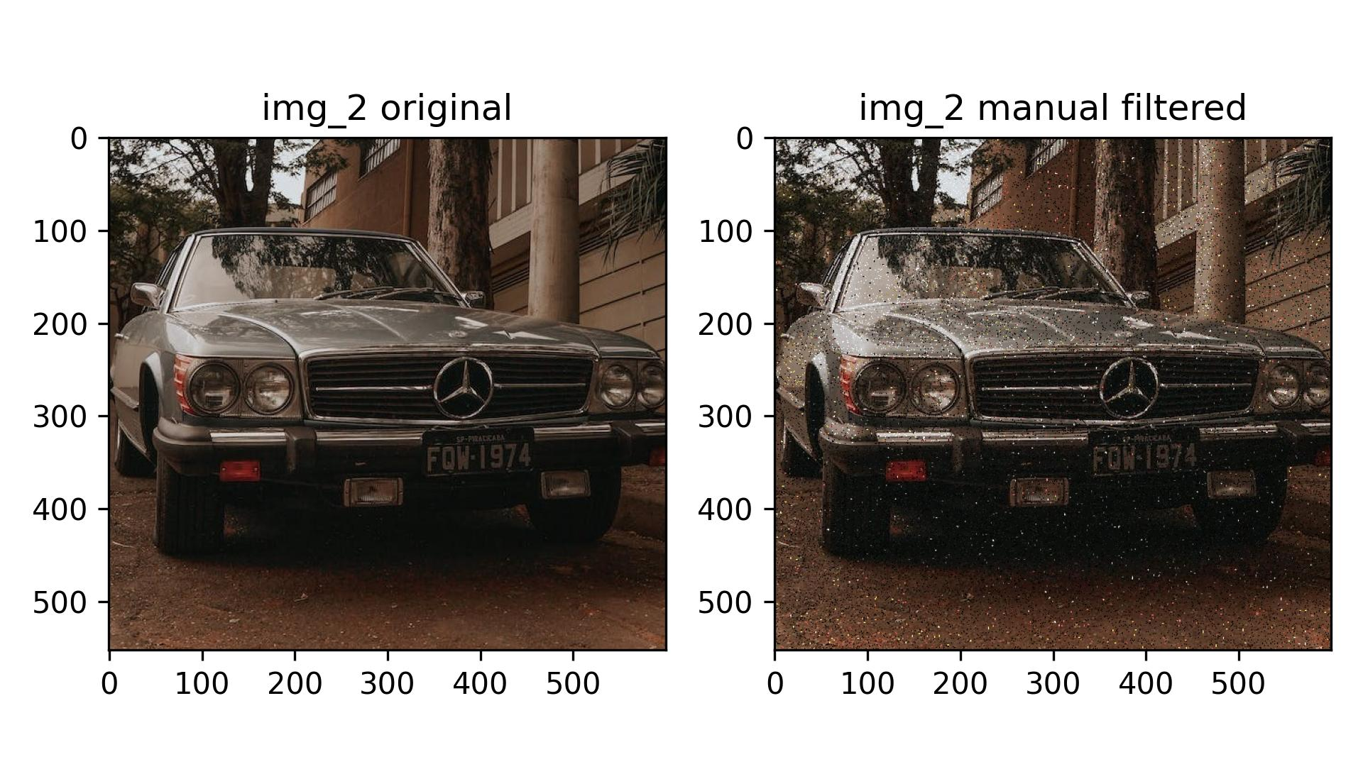
In addition to the median filter, we have developed a custom noise reduction method called the Variable Intensity Filter. This method is tailored to identify pixels with a significant difference from their neighbors and adjust their intensity accordingly.
Variable Intensity Filter: Implementation
import numpy as np

def variable_intensity_filter(img, threshold=150, weight=0.1):
    # Create a copy of the image to avoid modifying the original
    filtered_img = np.copy(img)

    # Iterate over each pixel in the image
    for i in range(1, img.shape[0] - 1):
        for j in range(1, img.shape[1] - 1):
            for k in range(img.shape[2]):  # Iterate over each color channel (RGB)
                # Calculate the average of neighboring pixels in the same channel
                neighbors_avg = np.mean([
                    img[i-1, j, k], img[i+1, j, k], img[i, j-1, k], img[i, j+1, k]
                ])

                # Calculate the difference between the current pixel and the neighbors' average
                diff = abs(int(img[i, j, k]) - int(neighbors_avg))

                # Adjust the pixel intensity if the difference exceeds the threshold
                if diff > threshold:
                    filtered_img[i, j, k] = int(img[i, j, k] * weight + neighbors_avg * (1 - weight))

    return filtered_img
Comparative Advantages
Our custom method offers several advantages:
- It targets only those pixels that significantly differ from their neighbors, preserving the image's overall integrity.
- The adjustable threshold and weight parameters provide flexibility, allowing fine-tuning based on specific image characteristics.
- This approach is particularly effective in images where noise is not uniformly distributed or is concentrated in specific areas.
Contrast Adjustment Techniques
Histogram Equalization Method
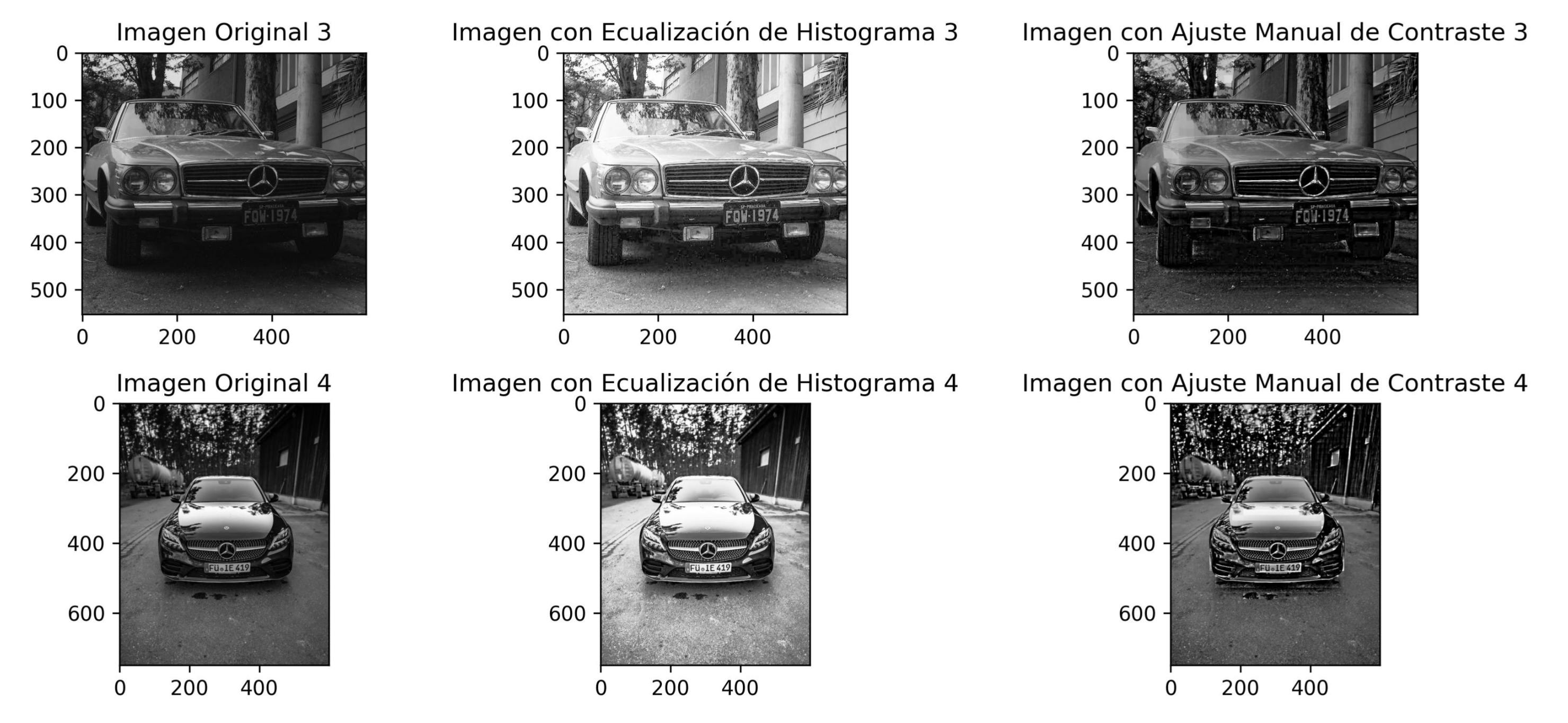
Histogram equalization is a widely used technique in image processing for improving contrast. It works by effectively spreading out the most frequent intensity values in an image, resulting in a more uniform distribution. By redistributing the brightness, histogram equalization can significantly enhance the global contrast, making the features more distinguishable.
OpenCV Implementation
import cv2 as cv

def histogram_equalization_cv(gray_image):
    return cv.equalizeHist(gray_image)
Our Custom Contrast Adjustment Method
Alongside standard techniques, we have developed a custom method for contrast adjustment.
This method, named adjust_contrast_weighted_local, focuses on locally adjusting the contrast based on a weighted scheme that considers both global and local mean intensities.
This approach allows for a more nuanced and detailed enhancement of image contrast, especially in images with varying lighting conditions.
Weighted Local Filter: Implementation
def adjust_contrast_weighted_local(image, factor, grid_size):
    img_float = image.astype(float)
    global_mean = np.mean(img_float)
    img_contrast = np.zeros_like(img_float)

    for i in range(0, image.shape[0], grid_size):
        for j in range(0, image.shape[1], grid_size):
            grid = img_float[i:i+grid_size, j:j+grid_size]
            local_mean = np.mean(grid)
            global_influence = global_mean / local_mean if local_mean != 0 else 1

            grid_contrast = local_mean + (grid - local_mean) * factor * global_influence
            img_contrast[i:i+grid_size, j:j+grid_size] = grid_contrast

    img_contrast = np.clip(img_contrast, 0, 255)
    return img_contrast.astype(np.uint8)
Comparative Advantages
Our custom method offers several advantages:
- This technique provides a more localized contrast enhancement, making it suitable for images with uneven lighting or exposure.
- The use of weighted factors based on local and global means allows more natural-looking results.
- It's particularly effective in bringing out details in both shadows and highlights.
Measuring Performance
Metrics for Noise Reduction
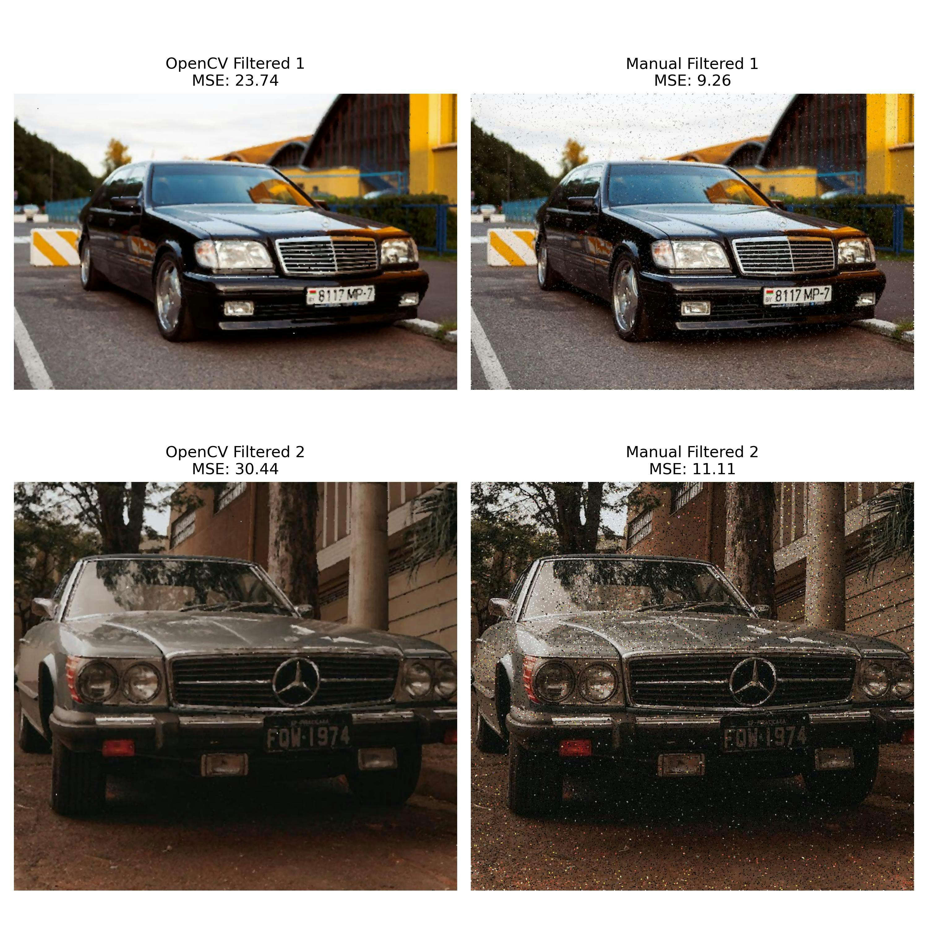
To quantify the effectiveness of our noise reduction techniques, we employ the Mean Squared Error (MSE). This metric measures the average squared difference between the original image and the processed image. A lower MSE value indicates a noise reduction technique that more closely approximates the original image, implying better performance.
def mse(imageA, imageB):
    return np.mean((imageA - imageB) ** 2)
Comparative Analysis
Using this function, we've calculated the MSE for images processed with both OpenCV and our manual filtering method. The results are as follows:
| Method | Execution Time | MSE | Best MSE |
|---|---|---|---|
| OpenCV Filtered 1 | 15ms | 23.66 | ❌ |
| Manual Filtered 1 | 5.5s | 10.03 | ✅ |
| OpenCV Filtered 2 | 15ms | 30.60 | ❌ |
| Manual Filtered 2 | 7.5s | 11.11 | ✅ |
Metrics for Contrast Adjustment
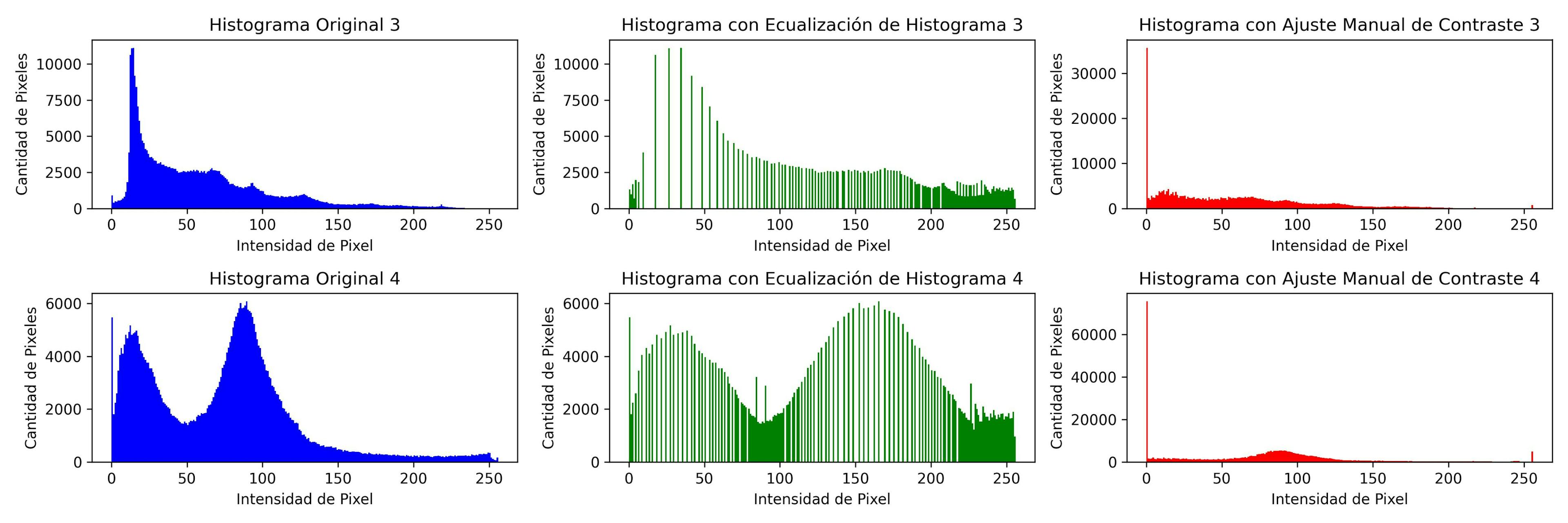
For assessing improvements in contrast, we visualize the changes in the histogram. Histograms provide a visual representation of the distribution of pixel intensities in an image, and are an insightful way to observe contrast adjustments.
We utilize the following code to plot histograms in Python:
import matplotlib.pyplot as plt

def plot_histogram(image, title, color):
    plt.hist(image.ravel(), 256, [0, 256], color=color)
    plt.title(title)
    plt.xlabel('Pixel Intensities')
    plt.ylabel('Number of Pixels')
Comparative Analysis
- Histogram equalization and our custom method both improve contrast visibly.
- Histograms from equalization show a broader distribution of pixel intensities.
- Our method yields more balanced enhancement, evident in the histograms.
- See below for before-and-after images and histograms for both methods.
Histogram Comparison
Conclusion
In summary, this series has explored noise reduction and contrast enhancement in image processing. We've delved into techniques like median filtering and histogram equalization, as well as introduced custom methods that provide localized enhancements and maintain natural image characteristics. These advancements are vital in fields ranging from medical imaging to digital photography, where clarity and detail are essential.
References
- OpenCV Documentation
- Putra, R. D., Purboyo, T. W., & Prasasti, A. L. (2017). A Review of Image Enhancement Methods. International Journal of Applied Engineering Research, 12(23), 13596-13603.
- Ačkar, H., Almisreb, A. A., & Saleh, M. A. (2019). A Review on Image Enhancement Techniques. Southeast Europe Journal of Soft Computing, 8(1).
- Prabhavi Jayanetti. (2020, October 16). Remove Salt and Pepper Noise with Median Filtering. Analytics Vidhya.
- Szeliski, R. (2010). Computer Vision: Algorithms and Applications. Springer.
- Ortega Muñoz, J. F., & Rivera Valencia, C. E. (2015). Aplicación de un filtro adaptativo para minimizar el ruido en una imagen. Universidad del Cauca, Facultad de Ingeniería Electrónica y Telecomunicaciones, Departamento de Telecomunicaciones, Grupo de Investigación y Desarrollo Nuevas Tecnologías en Telecomunicaciones-GNTT.